When you have an effluent, do you really know what the discharge is or are you simply making a best guess? For that matter, do you know how the permit limits are set? In the United States, a discharge permit generally contains a few critical numbers: the daily maximum and monthly average. Under the Clean Water Act’s latest revisions, noncompliance can lead to substantial penalties — potential fines of $2,500 to $25,000 per day of violation or a year in jail or both, with each day of noncompliance counting as a separate offense in civil or criminal actions.
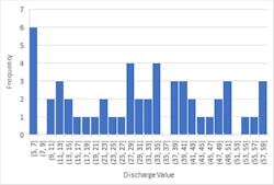
Figure 1. Upper and lower 95.5% confidence intervals fall outside the range of the sample population.
This underscores the importance of determining your permit limits at the time the permit is issued. You should identify and agree upon the type of statistical distribution applied in setting the permit limits.
Water quality standards generally set the maximum amount of contaminants you legally can discharge. The minimum discharge may not be zero even when the facility is shut down due to environmental and non-process related factors such as groundwater or contaminated stormwater on the site.
Conditions beyond a plant operator’s control can disrupt industrial and municipal treatment systems; these minor and major upsets can cause permit violations. The maximum amount of contaminants discharged is limited only by the size of the initiating event, the type of contaminant, the effect on the wastewater treatment system, environmental factors (rainfall, snowmelt, firewater discharges, etc.) and the operator’s ability to intercept and stop the event.
Some wastewater discharge permits are based upon a lognormal distribution for toxics, and a student’s T or normal distribution for “conventional” contaminants. (While some minor differences exist between the student’s T and normal distributions, here we’ll treat them as interchangeable.) Generally, the daily average discharge is a factor of two times the monthly average. With a standard normal distribution for conventional pollutants (BOD5, TSS, NO3, etc.), the daily maximum is set at two times the standard deviation on either side of the mean (monthly average) value. The two times standard deviation is supposed to represent 95.5% of the values of the population of possible discharges. But is this realistic?
A Telling Example
Let’s consider a population of 51 random numbers between 5 and 60 representing typical effluent concentrations (in mg/l) from a waste treatment plant discharge for a period of two months. Figure 1 depicts the frequency of 51 random values which represent discharge concentrations from a wastewater treatment plant for a 51-day period. The values were grouped for clarification, rather than listing all 51 values. For example: a number between 37 and 39 appeared three times in the sample, and there were no numbers in the intervals of 7–9, 35–37, and 51–53. If we use “conventional” statistics, the average of the discharges is 30.73 mg/L. The standard deviation of the population of discharges is 15.85 mg/L. That means that 95.5% of all possible discharges from a facility would be between -0.975 mg/L and 62.44 mg/L. The upper and lower 95.5% confidence intervals are outside the range of the population. So, what’s happening?
The idea is that over time an equal number of data points will fall above and below the mean — but they won’t. This distribution violates rationality because no facility can have a negative discharge value and discharge values significantly below the mean are rare (and highly improbable, some operators and engineers would say).
A wastewater treatment plant’s lower discharge value may approach zero but the maximum discharge value most often is beyond the operator’s control and depends on outside influences such as spills, rainfall, industrial chemicals in the influent, etc.
A lognormal analysis of the effluent data shows us a slightly better situation. The lognormal distribution is prepared using normal distribution procedures, except that Log10(x) or ln(x) replaces x in the population construction. The lognormal distribution boasts the advantage of having no negative values.
A lognormal distribution also has a fat upside tail, meaning a more forgiving and larger daily maximum discharge value. This also is true of a Weibull distribution. Equation 1 shows the probability function, X, for a lognormal distribution:
X = e(µ + σZ) (1)
where Z is a standard normal distribution variable, σ is the standard distribution and µ is the mean of the population of the variable’s natural logarithm. You can evaluate the parameters of the lognormal distribution once you know σ and µ, which often are referred to as the scale (β) and location (α) parameters. Running a lognormal analysis of our sample population gave β = 0.6992 (±0.2812) and a α = 3.2335 (±0.3893). From that, you can construct the probability density function and cumulative density function for the sample. The distribution has a correlation coefficient, R2, varying between 0.96 at lower values and 0.64 at higher values.
Weibull Distributions
Equation 2 shows the Weibull distribution:
f(x) = (β/α)(x/α)β-1exp(-[x/α]β) (2)
where α is the scale parameter and β is the shape factor. While Equation 2 looks formidable, it is very easy to compute.
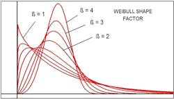
Figure 2 illustrates the different type of curve shapes obtained through Weibull analysis.
Figure 2. Shape factor, β, significantly affects the contour of the curve.
When the shape parameter β exceeds 1, the curve begins to resemble a standard distribution. At β = 3.44, the distribution looks like a lognormal distribution. Values above 4 start to indicate a specific type of material or equipment failure. The shape parameter of the distribution can provide information about failure modes — and, indeed, is widely used for evaluation of failures and preventive maintenance on a broad variety of process equipment. You certainly could argue that treatment plant systems depend upon the reliability of their mechanical equipment and, thus, a Weibull analysis is relevant.
A Weibull distribution features a longer right tail and fits the data. It could be an ideal way to establish permit limits when a facility is starting up or already running. A Weibull analysis will simulate normal, beta, lognormal and Weibull distributions based on your data. You can use inexpensive statistical programs and spreadsheets to calculate a Weibull distribution. A number of websites and online papers discuss the application of the Weibull distribution.
For our example, the Weibull distribution determined the following coefficients: β = 2.010 and α = 34.61. The correlation coefficient for the distribution is 0.9531 and varies from 0.89 at lower values to 0.97 at higher values, which is better than the lognormal distribution.
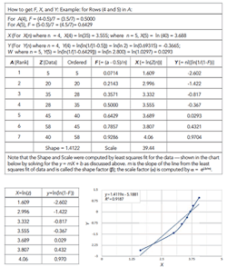
The linearity of the data points, as shown by the straight lines in the quartile-quartile plots in Figure 3, illustrates the goodness of fit of the Weibull and lognormal distributions.
Creating A Weibull Distribution
Two easy procedures exist for creating a Weibull distribution of your data using a spreadsheet. The first involves using the Weibull distribution function of the spreadsheet itself. Enter the data in column form, arrange the data from smallest to largest values, specify the range on the built-in software, and let the software do the work.
The second procedure requires slightly more work but gives you control — but first select data points to remove zeros.
Start by sequentially numbering all your data points, 1 through n, and create a column we’ll call A with n number of rows. If you have 25 data points, n will go from 1 to 25. Enter the actual data in a second column we’ll call Z. Then, rank the Z data from smallest to largest. You may have to copy the data using the “paste values” command but you can use the software to order the data from smallest to largest.
Create a column F for calculating the rank of Z by computing individual numbers from column A into column F by the following formula:
F = (a – 0.5)/n (3)
where a is the rank number in column A. (The -0.5 prevents you from topping out the scale and can be omitted for very large data sets.)
Then, use another column we’ll call X to take the natural log (nl) of values of Z.
Create a column Y that contains the natural log of the natural log of 1/(1-F). For all values, use:
Y = ln(ln[1/(1-F)]) (4)
Plot Y versus X, making the natural log of Z the horizontal axis and the values of Y as the vertical axis. Make the natural log of Z the horizontal axis. You’ll come up with a series of points on a graph that will have some negative values on the vertical axis.
Use the software to plot a straight line through your data and give you the equation for that line. It will be in the form of y = mx + b, where m is the Weibull shape parameter β. (The value of b probably will be negative but that’s all right.) Also, have the software find the correlation coefficient.
Figure 3. Weibull distribution provides a better fit than lognormal distribution.
Now compute α by solving:
α = exp(-b/m) (5)
where exp is base e to get the scale parameter. Congratulations, you have created a Weibull plot that is mathematically rigorous.
Figure 4 gives some example data in the various columns of a spreadsheet for calculating a Weibull distribution as well as the resulting plot. Of course, a larger data set could provide different and more-accurate values.
One useful online resource for these calculations is www.wessa.net/rwasp_fitdistrweibull.wasp.
Probable Errors And Permits
Other challenges are to find out what you actually are discharging and to measure the discharge as accurately as reasonably practical.
The discharge is mass based and equals the concentration times the flow.
If uncertainties exist in the measurement of any of these parameters, you have a permit uncertainty or probable error. Sometimes, the uncertainty can be as large the measured value. The probable error in a measurement, M, is composed of individual and independent functions, f1… fn, per:
M = f1(x) + f2(x) + f3(x) + … fn(x) (6)
The total probable error in M is given by:
e2 = (e1dx/df1)2 + (e2dx/df2)2 + ... (endx/dfn)2 (7)
where en is the error of measurement in the individual parameter.
Most flowmeters, including magnetic and doppler devices, have an accuracy to within ±2% depending upon the meter technology and design. Weirs and open-channel flowmeters can have a probable error of up to 10% depending upon installation conditions.
For a specific case, you can estimate the accuracy of the permit measurement. For example, say, the total suspended solids (TSS) concentration is 10 mg/L and the wastewater flow is 11,880 m3/d as measured by your flowmeter. The published accuracy for a suspended solids test according to standard methods is 15%. The measured discharge 118.8 kg/d.
If the flowmeter is accurate to within about 2% and the laboratory is accurate to within 15% on the particular test, then the relative error is
e = (0.152 + 0.022)½ = 0.15132 or 15.13%.
At the specified conditions, this error means your discharge could be anywhere between 100.1 and 135.85 kg/d. Similarly, if the reading is close to your maximum permit value, you actually could be over or under.
Figure 4. This illustrates the entries in the columns on the spreadsheet and the resulting graph.
The value of the error will vary with the accuracy of each of the individual parameters; you can reduce that error by multiple sampling or detailed analysis using the partial differentials above. Multiple analysis of the TSS will have great impact because the probable error decreases by the square root of the number of analyses.
There are a number of other errors in sampling; most of them depend upon the sampler. You might assume that the samples you collect are representative but they may not be. The U.S. Environmental Protection Agency (EPA) explored the issue of sampling devices and accuracy (“Sampling of Water and Wastewater,” EPA-600/4-77-036, August 1977, (page 16). Its efforts indicated that the ratio of the composite sample concentration to actual concentrations could vary between a low of 68% to a high of 135% depending upon the sampler and flow conditions. Most of the samplers averaged between 90 and 99% accuracy.
The U.S. Bureau of Reclamation’s publication “Water Measurement Manual” is an excellent reference for flow measurement and should be a part of every environmental engineer’s technical library; it is available online.
Accurate discharge measurement is a science and must be approached with accuracy and caution.
More information and a paper on sampling are available in the downloads section of my website: www.globalenvironmental.biz
DAVID L. RUSSELL, PE, is president of Global Environmental Operations, Inc., Lilburn, Ga. Email him at [email protected].
INTERESTED IN WASTEWATER TREATMENT?
Written by this article’s author, “Practical Wastewater Treatment” 2nd ed., published last year, provides an updated and expanded guide for handling industrial wastes and designing a wastewater treatment plant. For more details.
About the Author
David L. Russell
David is president of Global Environmental Operations, Inc. He is an experienced environmental/chemical engineer and has written on various subjects, including remediation, water and wastewater treatment, sampling and sustainability. He lectures and works in various parts of the world.


