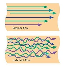
Fluid within the lines of an analytical sampling system exhibits one of two flow patterns — laminar or turbulent (Figure 1). Each type highly depends on the velocity of sample fluid as well as the fluid’s density and viscosity. It’s important to know the type of flow to expect when designing your system so you can make various adjustments to enhance the timeliness and accuracy of analytical measurements.
Turbulent flow typically is preferred in a sampling system. It enables faster analyzer responses and minimizes potential problems of contamination and clogging caused by settling of solids in sample lines. However, turbulent flow isn’t always achievable. Sometimes, you’ll have to accept the inherent deficiencies of laminar flow, including slower analysis.
To determine the type of flow to expect in your sample line, you must calculate the Reynolds Number, Re, to get an indication of the degree to which it is laminar or turbulent. If the value isn’t in the preferred range for your application, you may be able to manipulate some variables to achieve your desired flow.
Let’s review the differences between laminar and turbulent flow, how to calculate the Re, and some strategies for obtaining the desired flow for your sampling system.
Types Of Flow
Laminar flow occurs when the sample velocity is low. The flow is smooth, like a set of concentric cylinders of liquid slipping by each other. Running parallel to the sample line, each cylinder of fluid experiences a viscous drag from the cylinder just outside it — which slows down portions of the flow. The fluid at the center is traveling fastest while the fluid closest to the walls of the sample line is moving very slowly due to friction with the walls (Figure 1). The presence of this low velocity region may increase the response time for the slower moving fluid to reach the analyzer, particularly for liquid samples. Laminar flow is less detrimental to gas samples.
As sample velocity increases, the smooth laminar flow starts to break up and become more random, with some fluid movement across the radius of the sample line. Eventually, fully turbulent flow occurs. However, even when the flow is turbulent, a thin film of fluid close to the sample line walls still flows in laminar mode and may increase your response time slightly.
Turbulent flow promotes good sample mixing and clean sample lines because molecules are constantly moving and interspersing. It creates a fully mixed sample with all portions of the fluid traveling at about the same velocity in the line. Turbulence also enables faster analyzer responses, as the higher average velocity moves samples to the analyzer more quickly.
For these reasons, turbulence is desirable. However, it’s not essential. Sometimes, it’s not even practical, particularly if the high velocity required to generate turbulence causes excessive pressure drop or wasteful flow rates. These and other conditions may make laminar flow unavoidable. If so, you should design your system to provide the best flow possible, rather than limiting the flow to your desired response time. Doing so will provide the best possible response time under the constraints of the application.
Determining Flow Type
Because you can’t see inside your sample lines, to get an indication of the type of flow, you’ll need to rely on the fluid’s Re:
Re = D ρ u/η (1)
where D is internal diameter (m); ρ is fluid density (kg/m3); u is fluid velocity (m/s); and η is fluid viscosity (Pa∙s).
It’s often convenient to use a slightly modified version of this equation with noncoherent units:
Re = D′ ρ u/η′ (2)
where the diameter (D′) is in millimeters and the viscosity (η′) is in centipoise. These more common units still give the same value for the Reynolds Number.
An Re less than 2,000 typically means that flow is laminar. An Re of 4,000 or more indicates turbulence. An Re falling within the so-called critical zone between 2,000 and 4,000 may be laminar or turbulent.
Achieving Turbulence
When attempting to attain a suitable turbulent flow, you may need to adjust some variables in your sampling system, including the internal diameter of your sample lines and the fluid velocity.
In addition, you can manipulate the density and viscosity of the fluid by changing the pressure and temperature of the sample lines. Your ultimate goal is to increase the ratio of density to viscosity (ρ/η), thus favoring turbulence.
Rearranging Eq. 1 emphasizes the effect of the ρ/η ratio:
Re = D u × ρ/η (3)
This ratio is constant for a given process fluid running under controlled pressure and temperature conditions. So, it’s good to know how pressure and temperature influence the ρ/η ratio — and, therefore, turbulence — for both liquids and gases:
- For liquid samples, line pressure doesn’t significantly affect density or viscosity and, thus, turbulence.
- A rise in temperature usually reduces the viscosity of a liquid but has only a small effect on its density. Elevating the temperature, therefore, is likely to increase the Re and enhance the possibility of turbulence. Table 1 shows various parameters for water. If your liquid is viscous, a higher line temperature might help. The resulting reduction in viscosity will certainly boost the flow and may even initiate turbulence.
- For gas samples, increased line pressure doesn’t affect viscosity but compresses the gas, thereby raising its density. A higher pressure pushes up the ρ/η ratio, favoring turbulence.
- When heated, a gas expands and becomes a little less dense but its viscosity increases. Both factors reduce the Re. However, the net effect is relatively small as demonstrated in the values for air in Table 1. In practice, line temperature usually is set to avoid condensation of vapors without worrying about its effect on turbulence.
Other Design Choices
As noted above, velocity and line size also can influence the Re.
Looking at the ρ/η ratios in Table 1, let’s consider water at 25°C as an example. Its ρ/η ratio is 1.12 × 10⁶ s/m2. Let’s assume the velocity is at least 1 m/s, which is a typical minimum for sampling systems. In addition, let’s use ¼-in. × 0.035-in. tubing; it has an internal bore of 4.6 mm.
Inserting these numbers into Eq. 3 yields:
Re = 0.0046 m × 1 m/s × 1.12 × 10⁶ s/m2 = 5,200
At 5,200, the Re is above the turbulence threshold, even at a 1-m/s velocity. Using a smaller bore tube or lower velocity may push the Re below the desired threshold of 4,000 for turbulence. However, wider bore tubes are sure to be turbulent at the same velocity. So, you could raise the line size to increase turbulence — if that would enhance your analysis time or accuracy enough to justify the added material costs.
Now, let’s look at the numbers for a gas sample. The ρ/η ratios given in Table 1 are valid for air at 2 bara; you can see they’re much lower than those typical of liquid samples. Using the same sampling system setup as above and recalculating the Re at 25°C for air instead of water yields:
Re = 0.0046 m × 1 m/s × 1.26 × 10⁵ s/m2 = 580
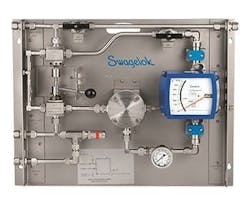
Therefore, the gas sample isn’t turbulent at this low velocity. It would take ¾-in. tubing running at 2 m/s to make this line turbulent; the vent flow rate then would be 47 L/min. To achieve this high flow rate, every component would have to be larger, and the sampling system would be costlier to fabricate. In addition, the large quantity of gas required for turbulence may be too valuable to flare, causing you to incur the additional cost of returning the gas to the process stream in a fast loop (Figure 2). You may opt for laminar flow in this case, so long as it won’t compromise sample analysis — and only if the lower flow of gas sample can be disposed safely.
Let’s take a quick look at some design strategies to achieve turbulence in gas samples.
To drive a gas sample into turbulence, you’ll need to raise line pressure, boost velocity or use a larger diameter line. Increasing the line size is the least effective strategy because doubling the line diameter will generate four times the flow rate. In contrast, doubling either the pressure or the velocity will generate only twice the flow rate.
Recalculating the ρ/η ratio when manipulating pressure is easy because gas density is directly proportional to its absolute pressure and its viscosity is unaffected by pressure. This means the ρ/η ratio will increase in proportion to gas pressure — and so, too, will the Re. For instance, consider the earlier gas example at the same velocity, but at seven times the line pressure. The ρ/η ratio and Re both now are seven times higher and the gas is turbulent:
Re = 0.0046 m × 1 m/s × 8.82 × 10⁵ s/m2 = 4,100
The flow rate also is seven times higher. Increasing the velocity by seven times yields the same result. Any combination of pressure and velocity that generates turbulence will produce the same vent flow rate and the same amount of waste gas.
If you plan to return the waste gas to the process, you can enhance turbulence by running the fast-loop supply line at full process pressure, being careful to maintain the line temperature above the process dew point to avoid condensation. Set the fast-loop flow rate to achieve the desired velocity in the supply line. The sample return line conditions are less important. However, try to maintain turbulence if you have a dirty sample. Allowing a dirty sample to drop into laminar flow might cause sedimentation and eventual blockage of your return lines.
Table 2 summarizes the Re obtained with typical line materials. Only samples with low ρ/η ratios, such as highly viscous liquids and low-pressure gases, need wide bore lines to achieve turbulence. Some heavy oils have ρ/η ratios less than 105 s/m2. They always will be in laminar flow mode unless you deploy wide bore tubing or piping and can tolerate the higher flow rate required.
Final Considerations
When designing your analytical sampling system, review the type of flow to expect in your sample lines by calculating the Re. If possible, shoot for an Re of 4,000 or greater to achieve turbulent flow and reap the benefits of faster sample analysis and better mixed samples. To obtain turbulence, you may need to manipulate various system parameters and operating conditions, such as sample line diameter, fluid velocity, pressure and temperature. When turbulence isn’t practical, laminar flow is acceptable, even though it may slow your response time. Check your options based on your ability to adjust the aforementioned variables, and recalculate the Re for each adjustment to arrive at the right design for your system and budget.
RANDY RIEKEN is market manager for chemical and refining for Swagelok Company, Solon, Ohio. Email him at [email protected].
MANAGING SAMPLE SYSTEM FLOW
This article is the second in a three-part series on the topic. It was adapted from “Industrial Sampling Systems: Reliable Design and Maintenance for Process Analyzers” (2013), a process sampling textbook authored by Tony Waters and published by Swagelok Company. For more information, visit www.industrial-sampling-systems.com.


