Improve control loop performance

Nearly all control loops in the chemical industry depend upon the manipulation of flow by the use of a final element such as a control valve. It’s generally taken for granted that when a controller changes its output, there’s an actual change in the position of the closure member of the valve (plug, ball or disk). However, the specification of control valves doesn’t adequately emphasize the very basic requirement that the position respond in a timely manner or even at all — and this has resulted in shortcomings that introduce variability into the process.
Before the advent of smart HART and fieldbus positioners, feedback measurements of position were rare because a separate position transmitter had to be purchased, installed and wired. So, the user generally wasn’t aware that differences in valve, actuator and pneumatic positioner design were the source of cycling in the process.
Typically, besides traditional factors such as size and materials of construction, control valve specifications have focused on minimizing leakage through the valve at shutoff and emissions to the environment from packing. Too often, to reduce project costs, plants pick on/off valves to address requirements. This can create performance problems that can’t be fixed simply by adding a smart positioner. While installing a smart positioner always is beneficial, an incorrect feedback mechanism in the valve design can give a false indication of performance.
To avoid problems, always consider five basic valve requirements — linearity, dead time, response time, resolution and dead band. They can give crucial guidance and justification for a final element that leads to better control. Rangeability and sensitivity also are important but, as we’ll see, properly meeting the other requirements will address them.
Linear in a nonlinear world
To get on a common basis, we need to define process gain for a self-regulating process as the final percent change in the controlled variable divided by the percent change in valve position. Note that the calibration span of the transmitter for the controlled variable is a factor. Because the changes seen in data historians for process variables are in engineering units, they must be converted to percent of scale. The maximum allowable controller gain is inversely proportional to the process gain.
The process gain for flow is the slope on a plot of percent flow versus percent valve position (travel). The plot should reflect the installed flow characteristic, not the inherent trim characteristic. This accounts for the reduced pressure drop available to the control valve at higher flows because of the increase in pressure drop in the rest of the system from frictional losses and a decrease in pump discharge pressure. The changing valve drop makes an equal-percentage trim more like a linear characteristic and a linear trim more like quick-opening characteristic. The effect increases as the valve pressure drop as a percent of the total system pressure drop is decreased.
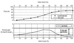
Figure 1. Process gain becomes too low when travel of sliding stem valve exceeds 80%. Source: Ref. 1.
In Figure 1, we see the process gain gets too low for travel above 80% of a sliding stem valve. The control loop must make very large changes in position to change the flow. For similar conditions a ball or butterfly with a 60° maximum rotation would see a corresponding excessive loss of sensitivity at about 60% travel, a typical problem for high capacity valves [1].
A linear installed characteristic is particularly desirable for flow and liquid pressure loops. For critical loops, software programs can generate the installed characteristics with normal fluid data used for sizing the valve if the system frictional loss and pump curve also are known. You then can set the controller gain per the maximum process gain on the plot. You can obtain better performance by computing the controller gain as a function of controller output per the plot. Of course, this depends upon a fixed installed characteristic, so in general the controller gain is reduced. An adaptive controller is now available that can automatically identify the process gain online for more accurate scheduling of the controller gain and tighter process control [2].
Another option is to put a signal characterization block between the controller output and the command signal for valve travel. The signal characterizer computes the percent stroke needed to obtain a percent desired flow (abscissa from the ordinate of the installed valve characteristic). This signal characterization will decrease the effect of resolution and dead band on the flat portion of the curve because it magnifies the change in signal to the valve. The opposite is true for steep portions of the curve. If control valve positions are maximized as plants are pushed beyond their design capacity, the greater concern is the loss in sensitivity at higher valve positions as shown in Figure 1.
If the pressure drop across the control valve is large compared to the pressure drop in the rest of the system — e.g., as in pressure letdown, reagent, surge and vent valves — the installed characteristic essentially is the inherent characteristic. For an equal-percentage trim, the nonlinearity is extreme (process gain can change by a factor of fifty) because the slope of the characteristic is proportional to flow. If a pH loop directly throttles a reagent valve on a static mixer, this change in slope on the valve characteristic compensates for a change in process gain for pH that is inversely proportional to flow.
For a temperature controller that directly throttles a coolant to an exchanger, the equal-percentage characteristic compensates for a temperature process gain that also is inversely proportional to flow. In either case, once a secondary flow loop is added so there’s a cascade loop of pH to reagent flow or temperature to coolant flow, we’re back to the nonlinearity considerations for the flow loop. Major reasons to add these secondary flow loops are to better reject pressure disturbances and provide a more accurate implementation of flow feedforward control [1].
A quick-opening trim characteristic provides initially a very high process gain followed by a very low process gain. This nonlinearity is accentuated in the installed characteristic and is generally undesirable because it magnifies resolution problems near the seat and causes an excessive loss of sensitivity even at mid-range throttle positions. Pinch valves and isolation valves designed for on/off service tend to have this characteristic.
Turning on a dime or at least a quarter
Dead time and response time quantify dynamic response. The dead time, Td, is the time to a first change in closure member position after a change in signal. The response time, T86, is the time required for the position to reach 86.5% of its final value and includes the dead time. These parameters are defined in the ISA standard and report for the test and measurement of the response of the complete control valve assembly [3, 4].
If you’re looking just at the actuator, you can estimate the pre-stroke dead time and stroking time from an individual fill or exhaust parameter for the actuator type and volume divided by fill or exhaust flow coefficient for the positioner, I/P or booster. The response time for large changes is estimated as 86% of the desired change in valve position (%) divided by the slewing rate (%/sec.). For changes between 1% and 10% the actuator response time becomes relatively fixed except for large valves and dampers.
It always was rather obvious that large valves were slow because it takes time to fill or exhaust enough air in a large actuator volume to make a change in actuator pressure large enough to overcome the torque or friction load to move the closure element. However, until recently, it wasn’t known that the response time of even small valves was dramatically slower, to the point of almost no response, because of the design of pneumatic positioners.
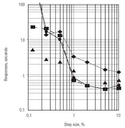
Figure 2. Various positioners on small actuators all exhibit much longer times for smaller step changes. Source: Ref. 3.
Figure 2 shows how the response time increases to 10 to 100 seconds from 1 to 2 seconds as the size of the step change in signal decreases below 1%. Note that in this plot we are primarily seeing the effect of the positioner because the step changes aren’t big enough to see stroking-time limitations. Spool-type positioners have an extremely slow response, to the point of no response for changes less than 0.2%. The response time for even good positioners can rise by an order magnitude for small steps.
HART and fieldbus digital positioners generally have eliminated this positioner resolution problem. When you also consider that pneumatic positioners tend to lose their calibration and have no position feedback or diagnostics, there’s considerable justification in terms of performance and maintenance for replacing such positioners.
In the days of analog control, a guideline advised using boosters instead of positioners on fast loops. With digital process loops and smart positioners, this no longer is an issue. It’s essential that every control valve have a smart digital positioner. A booster, if needed on a large actuator to reduce pre-stroke dead time and stroking time, should be installed on the outlet of the positioner with the booster bypass adjusted to prevent cycling by allowing the positioner to see a small portion of the actuator volume [5].
Achieving fine results
Resolution and deadband play a crucial role in valve response and highly depend upon the total valve package.
Resolution is the smallest change in signal in the same direction that will result in a change in position. Pneumatic positioners can adversely affect this but an even bigger potential problem originates from friction in the packing and seating through a behavior known as stick-slip where the valve closure member doesn’t move (sticks) and then breaks free and jumps to a new position (slips). Older designs of high-temperature and environmental packing as well as manual tightening of the packing beyond specifications can cause the resolution to deteriorate to 10% or worse.
A more insidious source of resolution problems is the high seat or seal friction particularly associated with valves designed for isolation. On/off (block) valves aren’t control valves and vice versa. If an application must prevent leakage, install an on/off valve whose action is coordinated with the opening and closing of a control valve. If a valve must operate near the seat due to rangeability requirements, it’s essential to ask the vendor for resolution measurements near the seat.
Don’t rely on stated resolution because this normally is for the valve at mid-position where the seating or sealing friction is lower. High friction and the discontinuity in process gains near the seat cause loops to oscillate around the split range point where there is a transition from one valve to another [6]. The realistic rangeability of a control valve (the largest flow divided by the smallest controllable flow) is set by the installed characteristic and resolution near the seat. Furthermore, repeatability isn’t as important as simply the ability of the valve to respond, as the process loop will correct for changes in the magnitude of the response.
Deadband is the smallest change in signal in the opposite direction that will result in a change in position. The deadband also is known as backlash and lost motion because it primarily originates from shaft connections and linkages. It’s particularly noticeable in rotary valves when there’s a translation of linear motion of an actuator to rotary motion of the ball or disk. Don’t count on rotary actuators as a solution; these actuators typically have been designed for on/off service and consequently don’t generally provide adequate resolution and deadband specifications. The effect is aggravated by high sealing friction and may result in shaft windup where the actuator shaft twists but the closure member is stuck and then considerably overshoots the desired position when it breaks free.
Particularly insidious on a rotary valve is a digital positioner feedback that uses actuator shaft position rather than closure member position because the positioner can think the valve moves when the ball or disk sticks. The response for Valve B in Figure 3 shows how such a positioner sees a change in position for step inputs of 1% when in fact the flow hasn’t changed until the step inputs are 5%. For some rotary on/off valves made into control valves by putting on a digital positioner, the actual deadband was 8% even though the smart positioner had extensive data showing the deadband was 0.5% [7].
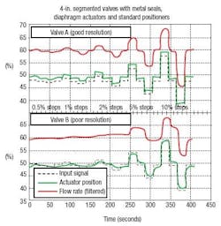
Figure 3. Even at mid-throttle the flow through Valve B only responds to larger-than-normal changes in the input signals.
Resolution and deadband add a dead time to the loop beyond that due to the actuator and positioner. This can be estimated as the resolution or half of the deadband divided by the rate of change of the controller output [1]. Resolution will cause a limit cycle (constant amplitude persistent oscillation) in any loop regardless of tuning [1]. For an integrating process such as level with a controller with integral action or a cascade control system where both the primary and secondary controller have integral action, deadband also will cause a limit cycle [8].
The amplitude of these cycles is the resolution or deadband multiplied by process gain for the process variable of interest [9]. For temperature and pH loops, this process gain can be 10 or more and can cause severe oscillations and process problems. Whereas problems from nonlinearity and response time are triggered by disturbances and tend to die out if the controller is properly tuned, limit cycles are continual. A digital positioner with good closure-member feedback that is tuned with a high gain and rate action can significantly reduce the amplitude of the limit cycles.
For pH control, the resolution of a reagent valve can determine the number of stages of neutralization needed. A small (fine adjustment) valve in parallel with a large (coarse adjustment) valve simultaneously manipulated by a model predictive controller can extend the sensitivity and rangeability of a reagent system enough to eliminate a stage [6].
Throttle your valve problems
A control valve package is only as good as its weakest link, whether it’s the actuator, positioner, feedback mechanism, packing or valve design. If the control valve and actuator are similar to those used for isolation valves, you’re a candidate for significant limit cycles (sustained variability) in your process. This is particularly a problem with packaged equipment (skids) where control valves are chosen based on piping specifications and lowest price rather than loop performance. Cost-effective solutions exist.
For example, a sliding stem valve designed for minimal seating friction and packing friction, coupled with a diaphragm actuator and a smart positioner, can reduce resolution and deadband to better than what you can achieve with a standard variable speed pump. Figure 4 shows that even operating near the seat a sliding stem control valve with a digital positioner can respond to changes as small as 0.1% (the smallest step listed in the ISA standard).
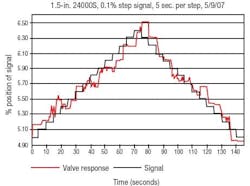
Figure 4. A sliding stem valve with a digital positioner can provide high resolution near seat.
References
- Blevins, Terrence L., "Advanced control unleashed,” ISA, Research Triangle Park, N.C. (2004).
- McMillan, Gregory K., "The next generation — adaptive control takes a leap forward,” Chemical Processing (Sept. 2004). Online at www.chemicalprocessing.com/articles/2004/145.html
- "Test procedure for control valve response measurement from step inputs,” ISA standard ISA-75.25.01-2000 (R2006), ISA, Research Triangle Park, N.C. (2006)
- "Control valve response measurement from step inputs,” ISA technical report ISA-75.25.02-2000 (R2006), ISA, Research Triangle Park, N.C. (2006)
- McMillan, Gregory K., "A funny thing happened on the way to the control room,” www.easydeltav.com/controlinsights/FunnyThing/default.asp
- McMillan, Gregory K., "A fine time to break away from old control valve problems,” Control (Nov. 2005). Online at www.controlglobal.com/articles/2005/533.html
- McMillan, Gregory K., Plant design category, http://ModelingandControl.com
- McMillan, Gregory K., "Life is a batch," Control (May 2005). Online at www.controlglobal.com/articles/2005/379.html
- McMillan, Gregory K., "What is your flow control valve telling you?," Control Design (May 2003). Online at www.controldesign.com/articles/2003/164.html
Gregory K. McMillan, is a principal consultant for Emerson Process Management, Austin, Texas. E-mail him at [email protected].