Don’t Get Duped By Deficient Data
The client was starting the design of a first-of-its-kind plant. One area involved vacuum flashing of a nominally dry chemical stream to generate as much vapor as possible. The feed to the vacuum flash came from a drum with a water boot. This prompted a question: Was the stream really dry or would it contain water and, if so, what effect would this have?
A search turned up only one datum for soluble water in the feed stream but it was at a different temperature. While getting more data at the correct conditions obviously was the best way forward, making a preliminary estimate of the water content certainly might prove helpful. There is a way to come up with such an estimate — but using it requires caution.
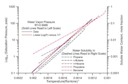
Figure 1 shows two families of plots. The first family is water vapor pressure (expressed as the log of absolute vapor pressure) versus reciprocal absolute temperature. The second family is soluble water content, in mole fraction, versus reciprocal absolute temperature. Note the scale for reciprocal temperature has been reversed so the direction of increasing temperature is from left to right.

Figure 1. Solubility does not relate simply to the number of carbon atoms in an alkane.
The water vapor pressure curve has an excellent fit to a straight line. There is some systematic bias — but across small temperature ranges this relationship is very accurate.
One way to think about the amount of a foreign phase that will dissolve is to imagine the immiscible liquid as an open space with some volume already taken by that liquid’s molecules. The amount of space the second liquid will occupy is proportional to its vapor pressure times a constant set by how much of the second liquid’s volume is “obstructed” by its own molecules.
This logic certainly holds true for soluble water in alkanes. Indeed, the second family of curves shows neat parallel lines for water solubility in propane, n-butane and n-hexane.
[callToAction ]
However, the second set of plots also highlights three areas for caution:
1. Comparing propane, n-butane and n-hexane, we see that water is most soluble in n-hexane, followed by propane and then n-butane. This points up that water solubility doesn’t necessarily behave simply with systematic changes in molecular structure in the same family.
2. As the mixtures approach their critical points, water solubility goes up dramatically and departs from the linear relationship of log mole fraction versus reciprocal temperature, as shown by the tail end of the curves on the upper right.
3. Different molecular structures create families of curves with different slopes. Propylene and benzene have more water solubility at low temperature and less water solubility at higher temperature than a constant linear relationship versus vapor pressure of water would predict. Structurally different molecules containing oxygen, nitrogen or other compounds can make the differences larger and less predictable.
If you only have one point, predicting water solubility a long way from your datum raises the risk of significant errors. If the errors have large consequences, you need more data.
In this case, with this client, the response to data uncertainty was to significantly increase the size of the equipment necessary to ensure processing capacity targets are met.
The project retained acceptable economics at the conceptual stage. However, the inevitable happened — a cost target was needed to offset some other changes. The question arose: How sure are you about the water solubility? The answer was not very sure; it could be better or worse. In this case, having good data is a possible cost-saving measure. Good data enable better equipment sizing if the basis used was too conservative. Good data allow for appropriate design to meet target capacities or better investment decisions if the basis used was too optimistic.
For simple molecular systems, two data points bracketing the processing range often will give good results. Three or four points bracketing the range will identify most non-ideal situations and allow for estimates sufficient for most uses. Nevertheless, be aware that some systems are extremely non-ideal and may require much more data.
